EDRM Statistical Sampling Applied to Electronic Discovery

Revised February 18, 2015

Contributors

Thanks to the following EDRM members, without whom Release 2 of Statistical Sampling Applied to Electronic Discovery would not exist:

• Michael Levine, principal author
• Gabe Luchetta, Catalyst
• Jamie LaMorgese, Catalyst
• Jeremy Pickens, Catalyst
• Rebecca Schwab, kCura
• Seth Magaw, RICOH
• Tony Reichenberger, Kroll Ontrack
• John Tredennick, Catalyst

Thank you also to Bill Dimm, Hot Neuron LLC, for additional comments and feedback.

1. Introduction

The purpose of this document is to provide guidance regarding the use of statistical sampling in e-discovery contexts. This is an update/enhancement of material that was originally developed and posted on the EDRM website in 2012.

E-discovery participants recognize that, when used appropriately, statistical sampling can optimize resources and improve quality. However, an ongoing educational challenge is to meet the needs of two audiences within the e-discovery community.

• Those who wish to improve their awareness of, and confidence in, these techniques without delving deeply into the technical math.
• Those whose e-discovery roles and responsibilities do require that they learn and understand the technical math.

Therefore, some of the material is covered twice. The earlier material is definitional and conceptual, and is intended for a broad audience. The later material and the accompanying spreadsheet provide additional, more technical information, to people in e-discovery roles who become responsible for developing further expertise.

The accompanying spreadsheet is EDRM Statistics Examples 20150123.xlsm.

• Download EDRM Statistics Examples 20150123.xlsm spreadsheet

1.1. Scope and Organization

As introductory matters, Subsection 1.2 provides a set of definitions related to statistical sampling, and Subsection 1.3 provides examples of e-discovery situations that warrant use of sampling.

Sections 2, 3, 4 and 5 examine four specific areas of statistics. The 2012 release focused only on the first of these, which is the problem of estimating the proportions of a binary population. If the observations of a population can have only two values, such as Responsive or Not Responsive, what can the proportion of each within a random sample tell us about the proportions within the total population?

The three new areas in this 2014 release are these.

• Quality control – using sampling to determine when the number of defects/errors is low enough to be acceptable.
• The particular problem of estimating recall. This has been an important issue in a number of e-discovery cases, e.g., da Silva Moore,[1. da Silva Moore v. Publicis Groupe SA, 11-cv-01279 (S.D.N.Y., filed 2/24/2011)(ESI Protocol and Order, Docket # 92, filed 2/17/2012).] Global Aerospace[2. Global Aerospace v. Landow Aviation, Va. Consol. Case No. CL 61040 (Va.Cir.Ct.Loudan Cty)(Order Approving the Use of Predictive Coding for Discovery, signed 4/23/2012).] and In re Actos.[3. In re Actos (Pioglitizone) Products Liability Litigation, 11-md-2299 (M.D.La., filed 12/29/2011)(Protocol Relating to the Production of Electronically Stored Information (“ESI”), Docket #1539, filed 7/27/2012).]
• Sampling for seed sets.

These topics are presented in basic, non-technical ways in Sections 2, 3, 4 and 5.

Section 6 presents some important guidelines and considerations when using statistical sampling in the e-discovery. These recommendations are intended to help avoid misuse or improper use of statistical sampling.

Sections 7, 8 and 9 are more technical. They present more formally the math that underlies the earlier material, and make use of the accompanying Excel spreadsheet.

1.2. Basic Statistical Concepts and Definitions

The purpose of this section is to define, in advance, certain terms and concepts that will be used in the ensuing discussions.

• Sampling – The process of inferring information about a full population based on observations of a subset of the population.
  • Sample – The subset is referred to as the “sample”.
  • Population – The total group from which the sample is drawn. Might also be referred to as the “universe”.
• Statistical sampling – Sampling that is done according to certain constraints and procedures, and thus conforms to certain mathematical models (“statistical models”) that can be used to quantify the implications of the sample observations for the total population. Randomness, defined below, is a key element of statistical sampling.
• Judgmental sampling – This term generally applies where a human decides what to include in the sample. For example, a human looks at the first five documents in a folder, or a human selects emails based on the subject line. The key point is that judgmental sampling that does not adhere to the constraints of statistical sampling, and thus cannot be used to reach the same quantitative conclusions as statistical sampling. Also known as informal sampling, intuitive sampling, or heuristic sampling.[4. In fact, even a machine could perform “judgmental” sampling if the machine has been programmed to find documents according to some non-statistical methodology.]
• Member (of the population) – Each individual unit or entity within the population.
• Observation – When a member of the population is selected for the sample, that member of the population is said to have been “observed”. The sample is comprised of observations.
• Attribute (of interest) – Members of a population, such as a collection of electronically stored documents, will have many characteristics or “attributes”. For example, date, file type, source/custodian. However, the purpose of statistically sampling is typically not to infer information about all of these. The purpose is typically limited to inferring information about one attribute of interest. In e-discovery, the attribute of interest is often “responsiveness”. Another example of attribute that may be of interest is whether the document is privileged.
  • As a general point, many attributes, such as dates and custodians, are easily known and aggregated by the computer. It is easy to know about these attributes for the full population. The purpose of sampling will typically be to learn about attributes that require some work to evaluate.
• Sample space – All the possible outcomes of an observation. More precisely, all the possible values of an attribute.
  • Where the attribute of interest is responsiveness, the possible values are “Responsive” or “Not Responsive”.
• Binary – When a sample space has only two possible outcomes (True or False, Heads or Tails, Responsive or Not Responsive), the attribute can be referred to as “binary”. Another term for this is “dichotomous”.
  • It is not binary if there are three possible outcomes.
• Proportion(s) – In a situation involving a binary attribute, this refers to the percentage of each outcome.
  • The sample proportion(s) are the observed percentages within the sample, such as 60% responsive and 40% non-responsive. The sum has to be 100%.
  • We can also refer to the “underlying” population proportion(s) or the “actual” population proportion(s). This, of course, is the information that we do not know and are trying to estimate.
  • In this document, proportions/percentages might be expressed in decimal form as well as percentage form. E.g., “0.60” is the same as “60%”.
• Yield – In the e-discovery context, when classifying a population of documents as either Responsive or Not Responsive, “yield” refers to the proportion that is Responsive. Also referred to as “prevalence” or “richness”. The terminology of document classification is discussed further in Section 4.
• Randomness – An important theoretical concept in probability and statistics. When selecting an observation from a population, the selection process is random if each member of the population has an equal probability of being selected. Statistical techniques that justify drawing quantitative conclusions about a population from a sample of the population depend on the assumption that the sampling is random.[5. In the case of stratified random sampling, samples from the sub-populations must be random, as discussed in Subsection 6.5.]
  • True randomness is hard to implement in a computer application, because computer applications by their nature are algorithmic and deterministic. Indeed, true randomness is often undesirable because the application user might want to be able to repeat or rerun sequences of “random” selections.
  • Therefore, applications that make selections for sampling use techniques that mimic the effect of random selection, and are thus viewed as adequate where there is a mathematical assumption of randomness. The term, “pseudo-randomness” is sometimes used to describe these techniques.

1.3. The EDRM and Sampling

The EDRM provides a great overall guide as to the individual steps and processes of e-discovery. For purposes of outlining when sampling is important and how it can be effective, the particular portions are found in largely in the middle of the EDRM.

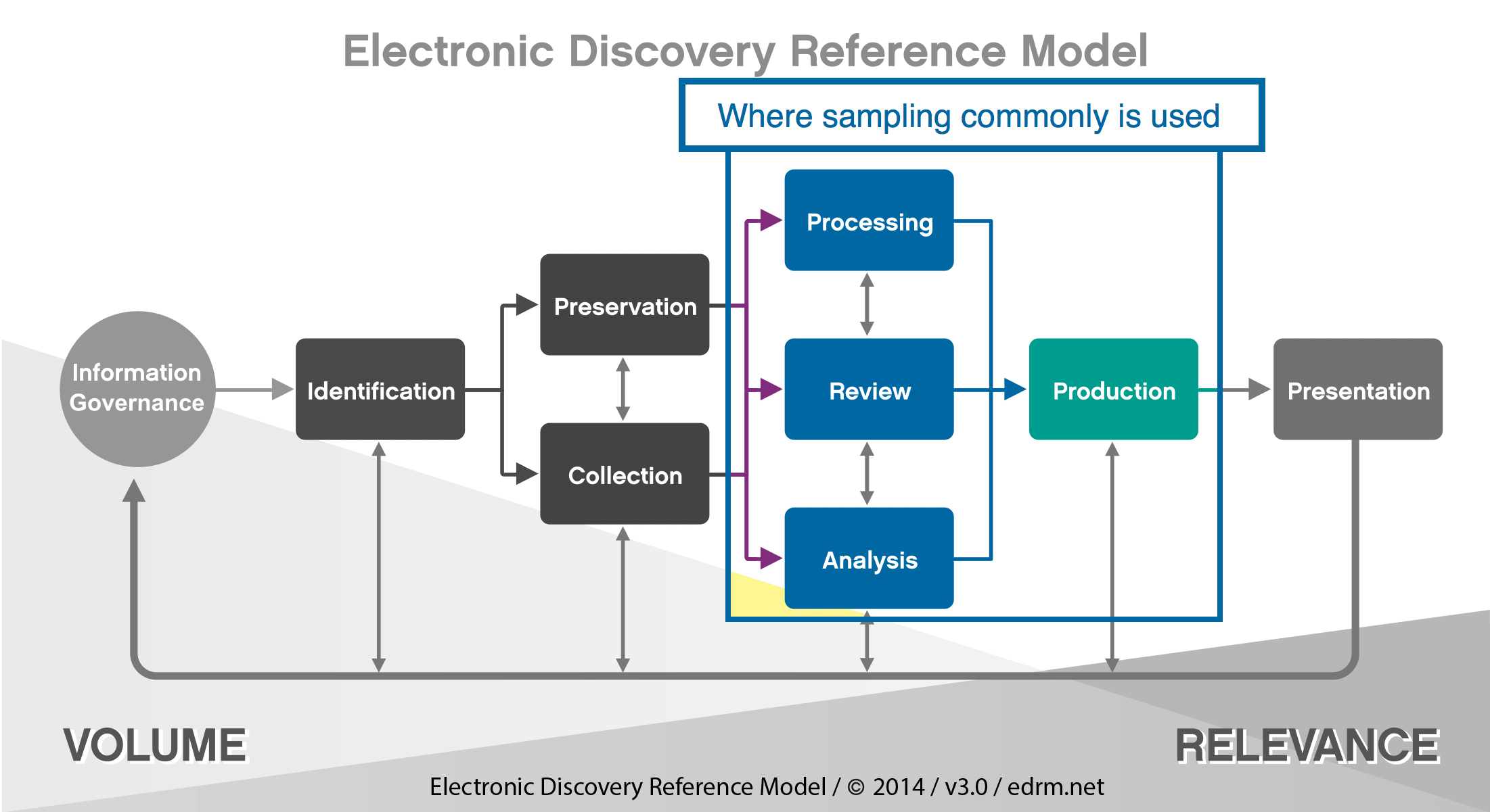
Generally speaking, the further to the left/top in the EDRM you are sampling, the more you are assessing inclusion of all material for review, the ability to review, the types of documents to review, and other items related to management of the process. The further to the bottom/right in the EDRM you go, the more you are assessing quality control and comprehensiveness of the process. Did you review everything you need to? Have you caught all privilege? Etc. Since the purposes differ, which impacts the method used to sample, it is necessary to address each portion separately.

• Sampling Prior to Review. While various forms of judgmental sampling may be used in collection of documents depending on the method of collection, it is rare to have statistical sampling of collections without review of some kind.[6. From a practical standpoint, sampling of collections in this context can’t happen without review. However, it is entirely possible that reviewing a sample of documents can lead to further collections based on it uncovering additional issues, further persons of interest, or items not previously in scope.] For that reason, statistical sampling usually begins with Processing.
  • Assessing Processing Quality. The first instance where sampling can be effective is in determining how well documents have been processed to the standards you wish them to be. E-discovery vendors often have numerous options in how documents are processed and require client input on these items. A small sample following processing can capture instances where the vendor erred or misunderstood the processing instruction, the client did not understand the impact of certain decisions or documents did not process correctly requiring re-processing ESI. If a number of documents were scanned into a database, this is also where you can assess how well the scanning was conducted, and/or how well OCR was applied.
  • Assessing File Types. Once data has been processed, often the next step is assessing what kind of data is available. At this point, identifying file types and extensions are helpful; in this regard, sampling a portion of various file types can influence how documents are to be reviewed (e.g. audio, multimedia documents), what documents can be removed from review (e.g. program files for instance).
  • Assessing Keywords/Filters. Data culling often occurs prior to review at this point. E-discovery practitioners often consider various keyword filters, date filters, and other means of reducing data to review. Many vendors consult and offer reporting from tools regarding the effectiveness of such filters; for instance, how many documents hit on a keyword, and if the particular document hit on other keywords used. In most cases, practitioners will have to defend their decisions on filtering and potentially validate the defensibility of those filters. Sampling at this phase can be extremely helpful in honing those filters to ensure that everything necessary is captured while reducing the number of false positives to the keyword hits. ESI Sampling from the universe of documents that were outside of the keyword results search (negative results) can provide further guidance to the case team on the quality of the search strategy. Using sampling, a case team may estimate the percentage of material defects, actual relevant documents, in the negative population. The case team may use this insight to expand the keyword terms to capture additional relevant documents.
• Sampling During Review. Statistical sampling during review can be helpful in two major aspects: 1) sampling to help provide review estimates; and 2) as a quality control measure to ensure that the categorizations are being properly applied.
• Sampling to Help Provide Estimates. Estimates of the time to review, the potential documents to produce, and the potential costs of a document review can sometimes be difficult to ascertain. Often, other reviews of similar content cannot provide comparable parameters for estimations on the current review because each case can vary so much. The number and scope of different issues, as well as the amount of documents appropriate to each issue, may make it impossible to estimate a current review from a previous review outcome. This is where an early statistical sample may be beneficial. A statistical sample early in the process can help gauge a number of factors that will help someone managing an e-discovery project assess how the project will go. For example, a simple estimate of the proportion of responsive documents in a collection (i.e., the yield or prevalence as defined above) can help estimate how many documents ultimately will be produced. Also, the amount of time it takes a reviewer to complete a sample can provide a basis from which to estimate completion of the database as a whole. In addition, for many e-discovery tool features, a statistical sample is necessary in order to assess the effectiveness of such features.
• Sampling as a Quality Control Measure. A case team may use sampling to estimate the quality of particular reviewers or an entire review team’s documents decisions when performing manual review. Sampling for the purpose of quality control can particularly benefit from Acceptance Sampling techniques, as discussed in Section 3.
• Sampling at the End of Review. Regardless of the method of review used, the question remains: When to terminate the review? Two Federal Rules of Civil Procedure are important here. Rule 26(b)(2)(C)(iii) limits discovery if “the burden or expense of the proposed discovery outweighs its likely benefit, considering the needs of the case, the amount in controversy, the parties’ resources, the importance of the issues at stake in the action, and the importance of the discovery in resolving the issues.” Rule 26(g)(1)(B)(iii) requires that discovery be “neither unreasonable nor unduly burdensome or expensive, considering the needs of the case, prior discovery in the case, the amount in controversy, and the importance of the issues at stake in the action.” The stronger the case that further review would be expensive, fruitless and disproportionate, the better the argument for ending the review. Any decision to end review early needs to be backed up with appropriate facts that justify this choice and generally, no single factor will be determinative on its own. However, demonstrably valid statistics can be one of the factors used to justify this decision. (The final decision to end review always rests with the client, their attorneys and the court, and it is not the purpose of this paper to suggest otherwise. The main point is that use of statistics can be part of the defensibility of that decision.)

2. Estimating Proportions within a Binary Population

One basic reason to use statistical sampling is to develop an estimate of proportions within a binary population. In addition to the estimate, itself, we want to quantify our “confidence” in the estimate according to established standards. This section provides a common-sense, intuitive explanation of this process. It presents the main concepts and provides some useable specifics, but without formal math. Formal math is presented in Sections 7 and 8 for readers who are interested.

2.1. Common Sense Observations

One need not be a math major or a professional statistician to have an intuitive appreciation of the following.

• In order to estimate the proportions of some attribute within a population, it would be helpful to be able to rely on the proportions observed within a sample of the population.
• Randomness is important. If you want to rely on a sample drawn from a population, it is important that the sample be random. This means that the sampling was done in such a way that each member of the population had an equal chance of being selected for the sample. As an example, in the political polling context if a pollster wants to sample from eligible voters in a state, the requirement of randomness is violated if the pollster only calls landlines. As another example, in an e-discovery document evaluation context, this requirement is violated if the sample is based only on the earliest documents in chronological order.
• The size of the sample is important. As the size of a random sample increases, there is greater “confidence” that the observed sample proportion will be “close” to the actual population proportion. If you were to toss a fair coin ten times, it would not be that surprising to get only 3 or fewer heads (a sample proportion of 30% or less). But if there were 1,000 tosses, most people would agree – based on intuition and general experience – that it would be very unlikely to get only 300 or fewer heads. In other words, with the larger sample size, it is generally apparent that the sample proportion will be closer to the actual “population” proportion of 50%.
• While the sample proportion might be the best estimate of the total population proportion, you would not be very confident that this is exactly the population proportion. For example, assume a political pollster samples 400 voters and finds 208 for Candidate A and 192 for Candidate B. This leads to an estimate of 52% as A’s support in the population. However, it is unlikely that A’s support actual in the full population is exactly 52%. The pollster will be more confident saying that A’s actual support is somewhere between 47% and 57%. And the pollster will very confident saying that A’s actual support is somewhere between 42% and 62%. So, there is a tradeoff between the confidence and the range around the observed proportion.

The value that math adds is that it provides a standard way of quantifying and discussing the intuitive concepts of confidence and closeness, and relating these to sample size.

2.2. Explanation of Statistical Terminology

Building on the preceding example involving political polling, the standard terminology for presenting the population estimate would be something like this:

Based on the sample size of 400 voters, A’s support is estimated to be 52% with a confidence level of 95% and a margin of error of ±5%.

Can we decode this?

• Sample size is just what it says – the number of observations in the sample.
• Margin of error of ±5% means that the pollster is referring to a range of 5% in each direction around the sample proportion. The range in this case is from 47% = 52% – 5% to 57% = 52% + 5%.
  • It is also possible to state the conclusion by simply stating the range, and without using the term “margin of error”: “Based on the sample size of 400 voters, A’s support is estimated to be in the range from 47% to 57% with a confidence level of 95%.”
  • When presented this way, using an explicit range, the explicit range is referred to as a confidence range or confidence interval. As compared to the margin of error, the confidence range has the advantage that it does not have to be exactly symmetrical around the sample proportion.
• This leaves the term, confidence level. Obviously, 95% sounds pretty good. 98% or 99% would sound even better. Is 95% high enough? 90%?
  • Here is the derivation of the confidence level concept: The pollster in our example took a sample of 400 from the underlying population. That was just one of a very large number of “size 400” samples that could have theoretically been drawn from the population. When we say that the confidence level in this case is 95%, we are saying that 95% of the theoretically possible “size 400” samples are within 5% of the actual proportion. Thus, we are saying that 95% of the time, any particular “size 400” sample that is actually selected will be within 5% of the actual proportion.

One further definitional point that bears repeating is that the margin of error is a proportion of the population, and not a proportion of the estimate. Using the political polling example above, where A’s support is estimated to be 52% with a confidence level of 95% and a margin of error of ±5%, assume the sample is from a voting population of 10 million. The 52% sample proportion leads to a “point estimate” within the population of 52% of 10 million = 5,200,000 million. Applied to the population, the margin of error is ±5% of 10 million = ±500,000 and the confidence interval is from 4,700,000 to 5,700,000. It is not correct to say that the margin of error is ±5% of the 5,200,000 point estimate, or ±260,000.

2.3 Sample Size, Margin of Error and Confidence Level are Interdependent

Without getting into the math, it is fair to say – and hopefully intuitively obvious – that sample size, margin of error/confidence range and confidence level are interdependent. You want to increase the confidence level, but that requires increasing the sample size and/or increasing the margin of error. This creates tradeoffs, because you would prefer to reduce the sample size (save time and work) and/or reduce the margin of error (narrow the range).

Following are two tables that illustrate this interdependence. (These tables are derived using a very basic technique, as discussed briefly in Subsection 2.4, and then more fully discussed further in Section 8, and the accompanying spreadsheet.[7. The method used to create the tables is technically referred to as a “Wald approximation” that assumes an underlying population proportion of 50%. See Section 8.])

Table 1 shows different possible “pairs” of margin of error and confidence level assuming sample sizes of 400 and 1,500.

Table 1
Sample Size	Margin of Error	Conf Level
400	0.0100	0.3108
400	0.0200	0.5763
400	0.0300	0.7699
400	0.0500	0.9545
400	0.0750	0.9973
400	0.1000	0.9999
1,500	0.0100	0.5614
1,500	0.0200	0.8787
1,500	0.0300	0.9799
1,500	0.0500	0.9999
1,500	0.0750	1.0000
1,500	0.1000	1.0000

The pollster who reported a 5% margin of error with a 95% confidence level on a sample size of 400 was reporting consistently with the case highlighted in green, allowing for conservative rounding. With a sample size of 400, the pollster could have just as accurately reported a 2% margin of error with a 57% confidence level or a 10% margin of error with a 99% confidence level. Once you have results for a sample of a given size, you can equivalently report small margins of error (tight ranges) with low levels of confidence, or large margins of error (wide ranges) with higher levels of confidence.

Table 1 also shows that increasing the sample size will reduce margin of error and/or increase confidence level.

Table 2 shows the required sample sizes for different standard values of margin of error and confidence level.

Table 2
Conf Level	Margin of Error	Sample Size
0.9000	0.0100	6,764
0.9000	0.0200	1,691
0.9000	0.0500	271
0.9000	0.1000	68
0.9500	0.0100	9,604
0.9500	0.0200	2,401
0.9500	0.0500	385
0.9500	0.1000	97
0.9800	0.0100	13,530
0.9800	0.0200	3,383
0.9800	0.0500	542
0.9800	0.1000	136

The highlighted combination shows that the required sample size for an exact 95% confidence level and 5% margin of error is actually 385.

2.4. Situations Involving Proportions Close to 0 or 1

Consider a situation where 385 electronic documents are sampled for relevance to a particular discovery demand and only three documents are relevant. The sample proportion is thus only 3/385 = 0.007792 = 0.78%. Using Table 2, this would imply a 95% confidence level with a margin of error of ±5%. The confidence range would this be calculated as from 0.78% – 5% = -4.22% to 0.78% + 5% = 5.78%, and this of course makes no sense. The population proportion cannot possibly be negative. Also, since there were some relevant documents in the sample, the population proportion cannot possibly be zero.

There would be a similar problem if there had been 382 relevant documents in the sample of 385.

This is a practical example that illustrates the limitations of the math behind Tables 1 and 2. Another mathematical approach is needed in these situations, and fortunately there are approaches that work. Using one of the more common techniques,[5. Technically referred to as the Clopper-Pearson version of the binomial exact method. See Section 8.] we can say that the estimated population proportion is 0.78% with a 95% confidence level and a confidence range from 0.17% to 2.32%.

Notice that this confidence range is not symmetrical around 0.78%. (0.78% – 0.17% = 0.61% while 2.32% – 0.78% = 1.54%.) This not a case where we can use the term (or concept) “margin of error” to indicate the same distance on either side of the sample proportion.

Thus, it is important to remember that

• The math behind the simple explanations and examples, such as those is in the previous subsection, is really just introductory material from a mathematician’s perspective.
• There are a number of more advanced techniques -– and alternatives within techniques — that can and often should be employed in real world contexts involving proportion estimation.

If we explain only the simple math, we leave the incorrect impression that this is all one has to know. If we explain more, we go beyond what most non-mathematicians are willing to engage and digest. We resolve this dilemma by keeping things as simple as possible in Sections 2, 3, 4 and 5, and then providing more advanced material in Sections 7 and 8, and the accompanying spreadsheet.

3. Acceptance Sampling

Not every situation requires an estimate of the population proportions. In some situations, it is more important to be confident that the population proportion is zero or very close to zero than to develop an actual estimate. For example, if a set of 2,000 documents has been reviewed by a human reviewer, we might want to use sampling to develop a level of confidence that the human reviewer’s error rate is not worse than some pre-established tolerance level, such as 10%. Our concern is that the error rate not be 10% or more. Since we are not concerned with the question of whether the actual rate is 2% or 3% or 5% or whatever, this enables smaller sample sizes.

Sampling problems of this sort are addressed in an area of math known as acceptance sampling. This section provides a basic introduction. More formal math is presented in Section 9 for readers who are interested.

We can understand intuitively that if we take a sample of the documents, and there are zero errors in that sample, we can get some confidence that the total error rate in the population of 2,000 documents is low. In quantitative terms, the problem could be framed as follows.

• We will take a sample of the 2,000 documents.
• We will accept the human reviewer’s work if there are zero errors in the sample.
• Our goal is to have a 95% confidence level that the reviewer’s error rate is less than 10%.
• This means that, if the actual error rate is 10%, there is a 95% or greater chance that the sample will have one or more errors, so that we correctly reject the sample 95% of the time.
• So, how big must the sample be?

Acceptance sampling has developed as the mathematical approach to addressing these types of questions, and has traditionally been employed in the context of quality control in manufacturing operations. The types of underlying math are the same as those used on proportion estimation.

Table 3 shows the required sample sizes for different population sizes, confidence levels and unacceptable error rates. The row highlighted in green shows that a sample size of only 29 will meet the criteria in the example as posed.

Table 3
Pop Size	Conf Level	Unacceptable Error Rate	Sample Size
2,000	0.9000	0.1000	22
2,000	0.9000	0.0500	45
2,000	0.9000	0.0100	217
2,000	0.9500	0.1000	29
2,000	0.9500	0.0500	58
2,000	0.9500	0.0100	277
2,000	0.9800	0.1000	37
2,000	0.9800	0.0500	75
2,000	0.9800	0.0100	354
100,000	0.9000	0.1000	22
100,000	0.9000	0.0500	45
100,000	0.9000	0.0100	229
100,000	0.9500	0.1000	29
100,000	0.9500	0.0500	59
100,000	0.9500	0.0100	298
100,000	0.9800	0.1000	38
100,000	0.9800	0.0500	77
100,000	0.9800	0.0100	389

Rigorous quality control (“QC”) review using acceptance sampling might not have been a standard procedure in legal discovery in the past, especially when the entire coding was performed by humans. The advent of machine coding has increased the recognition that QC is a vital part of the e-discovery process.

This example shows what can be done, but also just scratches the surface. An important extension, using this example, is to find a sampling approach that also minimizes the probability that we mistakenly reject a reviewed set when the actual error rate it an acceptable level.

As noted, a more advanced technical discussion of acceptance sampling appears in Section 9.

4. Sampling in the Context of the Information Retrieval Grid – Recall, Precision and Elusion

For some time now, the legal profession and the courts have been embracing, or at least accepting, the use of technologies that offer the benefit of avoiding 100% human review of a corpus. Statistical sampling serves the important role of evaluating the performance of these technologies. After a brief discussion of key concepts and terminology, this section discusses the statistical issues that will be encountered and should be understood in these situations.

4.1. Concepts and Definitions

These concepts and definitions are specific enough to this section that it was premature to list them in Subsection 1.2. Different observers use some of these terms in different ways, and the goal here is not to judge that usage. The goal is simply to be clear about their meanings within this discussion.

• Context – As a reminder, the basic intent of the litigation review process is to understand and analyze documents and then to classify them. A fundamental form of classification is whether a document is responsive to an adversary’s discovery demands or non-responsive.[8. Some commentators discuss this subject using a relevant/not relevant distinction instead of a responsive/not responsive distinction. There is a difference in that, for example, a document could be probative with respect to an issue in the case (and thus theoretically relevant) but might not have been demanded in any discovery request (and thus not responsive). It is not the purpose of this material to dwell on these sorts of issues. The purpose is to get to the statistical methods that can assist whatever the classification is being applied.]
• Gold Standard – For the purposes of this discussion, we accept the proposition that there is a correct answer and that a properly informed human attorney – someone who is familiar with the case, the issues and the standards – will provide the correct answer. Thus, we sometimes refer to the human reviewers as the gold standard.
• Classifier – A classifier, really, is any process or tool that is used to classify items. For our purposes we are focusing on e-discovery processes and tools that classify documents and comparing the performance of these classifiers to gold standard human review. Obviously, the better the performance, the greater the willingness to use/accept the results and to forgo (presumably more expensive) full human review. It is emphatically not the purpose of this material to discuss or describe the different specific classifier tools, techniques and technologies that have been emerging. From a statistical validation perspective, it does not really matter whether the classifier employs “supervised machine learning” or a “rules based engine” or traditional keyword searches or any other approach or combination of approaches. The important goal is to measure how well the classifier performs, as compared to the gold standard human reviewer.
• The Information Retrieval Grid, aka Confusion Matrix, aka Contingency Table is, per Grossman and Cormack, “a two-by-two table listing values for the number of True Negatives (TN), False Negatives (FN), True Positives (TP), and False Positives (FP) resulting from a search or review effort.”[9. https://edrm.net/glossary/confusion-matrix/.]

		According to Gold Standard Human Expert (“Actual”)
		Responsive	Not Responsive	Total
According to Computer Classifier (“Predicted”)	Responsive	True Positive (TP)	False Positive (FP)	Predicted Response (PR = TP + FP)
	Not Responsive	False Negative (FN)	True Negative (TN)	Predicted Not Responsive (PN = FN + TN)
	Total	Actual Responsive (AR = TP + FN)	Actual Not Responsive (AN = FP + TN)	TOTAL (T)

• As presented, the Positive and Negative are from the perspective of the classifier. In this case, a document is a Positive if the classifier says it is responsive and Negative if the classifier says it is non-responsive. True and False are from the perspective of the gold standard human reviewer. If the classifier is correct per the gold standard, a Positive is a TP and a Negative is a TN. If the classifier is not correct per the gold standard, a Positive is a FP and a Negative is a FN.
• Three important measures based on this grid are
  • Precision – TP/(TP + FP) – The proportion of predicted responsives (positives) that actually are responsive.
  • Elusion – FN/(TN + FN) – The proportion of predicted non-responsives (negatives) that actually are responsive.
  • Yield – AR/T – Simply the proportion of all documents that are responsive, as previously defined in Subsection 1.2.
• We can use sampling to estimate precision, elusion and yield. This is just an application of proportion estimation for a binary population, as discussed in Section 2. The classifier generates the full positive and negative populations, and of course the total population is known even before application of the classifier.
  • If the classifier is working well (as hoped), precision will approach 1 and elusion will approach 0. Thus, the considerations set forth in Subsection 2.4 would apply.
• Recall – TP/(TP + FN) – is another important measure. Recall is the proportion of actual responsives that are correctly classified as responsive. Indeed, from the practical perspective of a demanding party, recall is arguably the most important measure. The demanding party wants to see all the responsive documents.

4.2. Confidence Calculations When Sampling for Recall

An important observation arising from the definitions in Subsection 4.1 is that sampling for recall presents a greater challenge than sampling for precision, elusion or yield.

When sampling for precision, the underlying population – predicted responsives – is a known population based on the work done by the classifier. Similarly, when sampling for elusion with an underlying population of predicted non-responsives and sampling for yield with the underlying population being the full population.

However, when sampling for recall, the underlying population – actual responsives — is not, itself, a known population until there has been gold standard review. As a result, and as will be explained, sampling for recall requires larger sample sizes than sampling for the other key metrics in order to achieve the same levels of confidence. We will discuss two common techniques for sampling for recall.

One technique has been referred to as the “Direct Method”.[10. Grossman, M.R, and Cormack, G.V, Comments on “The Implications of Rule 26(g) on the Use of Technology-Assisted Review, 7 Fed. Cts. L. Rev. 285 (2014), at 306, and sources cited therein.] The essence of the direct method is to sample as many documents as necessary from a full corpus to find a sample of the required size of actual responsives. Even though the AR population is not known, a sample of actual responsives can be isolated by starting with a sample from the full population and then using human review to isolate the actual responsives from the actual non-responsives.

Thus, the required amount of human review will depend on the yield. For example, if the intent is to estimate recall based on a sample of size of 400, and the actual responsives are 50% the total population, human reviewers would have to review approximately 800 (i.e., 400/0.50 documents) in order to isolate the 400 that could be used to estimate recall. (The number is approximate because the process requires review of as many documents as necessary until 400 responsives are actually found.)

Similarly, if the actual responsives are only 10% of the total population, human reviewers would have to review approximately 4,000 (i.e., 400/.10 documents) in order to isolate the 400 responsives that could be used to estimate recall.

This reality regarding sampling for estimation of recall was understood in In re Actos.[11. In re Actos (Pioglitizone) Products Liability Litigation, 11-md-2299 (M.D.La., filed 12/29/2011), Case Management Order: Protocol Relating to the Production of Electronically Stored Information (“ESI”), Docket #1539, (filed 7/27/2012).] The parties agreed that the initial estimate of yield (termed “richness” in the In re Actos order) would be based on a sample of size 500 (the “Control Set”).[12. Id. at 11.] They further agreed that the sample should be increased, as necessary, “until the Control Set contains at least 385 relevant documents” to assure that the “error margin on recall estimates” would not exceed 5% at a 95% confidence level.[13. Id. At 12.]

A second technique for estimating recall is based on expressing recall as a function of combinations of precision, elusion and/or yield. For example,

Precision = TP/Positives, so TP = Precision * Positives

Elusion = FN/Negatives, so FN = Elusion * Negatives

Recall = TP/(TP + FN), so Recall = (Precision * Positives) / (Precision * Positives + Elusion * Negatives)

We can estimate precision and elusion using binary proportion techniques, and then put those estimates into the above formula to get an estimate of recall.

However, it is not correct to say that this estimate of recall has the same confidence level as the individual estimates of precision and elusion. The additional math required to express the confidence levels and confidence intervals is beyond the scope of this material, but suffice to say that this type of approach will not necessarily or substantially reduce the overall necessary sample sizes relative to the direct method.

4.3. Elusion Testing as Alternative to Recall Calculations in a Low Yield Situation

In many situations, high recall will coincide with low elusion and vice versa. Since elusion is easier to sample than recall, for the reasons noted above, some commentators recommend elusion testing as an alternative to a recall calculation.

However, it is not always the case that the high recall/low elusion relationship will hold. For example, if a population has a 1% prevalence rate and the documents identified as non-responsive by the classifier have a 1% elusion rate, the classifier performed poorly. The classifier did not perform better than random guessing. Elusion would be “low”, but this would not indicate high recall.

Grossman and Cormack also reference this issue.[14. https://edrm.net/glossary/elusion/.]

5. Seed Set Selection in Machine Learning

Having stated in Subsection 4.1 that it is not the purpose of this material to discuss particular classification technologies, it is still useful to make one observation that updates/corrects a point made in the EDRM statistics materials from 2012.

In discussing the use of sampling to create a seed set for the purpose of machine learning, those materials stated that it is “recognized that it is important to the process that this sample be unbiased and random.” It is no longer appropriate, if it ever was, to make this generalization.

Basically, there are multiple approaches to machine learning. They do not all use the same algorithms and protocols. Different designers and vendors use different techniques. There may be approaches under which the use of a random seed set is optimal, but there also may be approaches under which some form of judgmental sampling is more effective. One might say that the optimal protocols for seed set selection are vendor specific.

This provides a good lesson in a basic point about sampling. Randomness is not an inherently good quality. Random sampling is not inherently superior to judgmental sampling. Random sampling makes sense when your goal is to apply some specific mathematical techniques (such as confidence intervals and acceptance sampling), and those techniques depend on the specific assumption of randomness. Random sampling does not necessarily make sense when your goal is to work within a framework that is predicated on different assumptions about the incoming data.

6. Guidelines and Considerations

While statistical sampling can be very powerful, it is also important that it not be used incorrectly. This section discusses some common sense considerations that might not be obvious to people with limited exposure to the use of statistics in practical contexts. The goal is to provide guidance addressed at preventing problems.

6.1. Understand the Implications of “Culling”

We can use the term “culling” to describe the process of removing documents from the population prior to review on the basis that those documents are believed to be non-responsive. Issues arise in the degree of certainty about non-responsiveness.

• There may be situations where there is high certainty that a category is non-responsive, but there is less than absolute certainly. For example, based on interviews with employees, documents associated with particular custodians or stored in particular locations. Counsel may conclude that no human review appears necessary, but it also may be appropriate as a matter of defensibility and good practice to use some strict (“zero tolerance”) acceptance sampling to confirm that belief. They would be removed from the main review population, subject to an unexpected finding in the acceptance sampling.
• There are forms of “culling” that really amount to classification and where false negatives are reasonably expected, albeit not many. An example here would be the use of a keyword search to reduce the population prior to a machine learning assisted review of the remaining documents. In this situation, statistical measures of the process, particularly recall, should take all of these documents into account.

6.2. Recognize When Your Standards Change

Practitioners understand that standards can change during review. It is entirely possible that what has been considered responsive or relevant has changed over the course of review.

It is possible, however, that the actual standards for responsiveness can change in the course of a review. This change in standards might be based on information and observations garnered in the early stages of the review. If this is case, then of course it would not be sound to use a sample based on one set of standards to estimate proportions under different standards.

Some calls are close calls. This does not, in itself, undermine the validity of statistical sampling, as long as the calls are being made under a consistent standard.

6.3. Be Careful in Comparing Deduplicated Results to Pre-Deduplicated Results

Do not assume that the proportion of responsive documents in a deduplicated population is the same as the proportion that had been in the pre-deduplicated population.[15. It is not the intent here to discuss different possible types of deduplication – exact matches, near matches, etc. In terms of statistics, the fundamental points are the same.] This would only be true if the deduplication process reduced the numbers of responsives and non-responsives by the same percentage, and there is ordinarily no basis for knowing that.

As a simple example, assume a pre-deduplicated population of 500,000, of which 100,000 are responsive and 400,000 are non-responsive, for a 20% yield rate. (Of course, these amounts would not actually be known prior to sampling and/or full review.) The deduplication process removes 50,000 responsives and 350,000 non-responsives, resulting in a deduplicated population of 100,000, of which 50,000 are responsive, for a 50% yield rate. (Again, these amounts would not actually be known prior to sampling and/or full review.)

This may seem like an obvious point, but it is worth repeating because it leads to some important lessons.

• When estimating proportions in a population, make sure all interested parties understand the exact definition of the population. For the example cited, the question, “What is the yield rate?” is ambiguous. Either answer, 20% or 50%, is correct for the associated population, but you must be explicit in defining the population.
• This same ambiguity should certainly be avoided when estimating recall, where the rate itself may be an important benchmark.
• Substantively, one can reason that it is more important to have a high recall rate within the deduplicated population than the pre-deduplicated population. The premise here is that the real goal is high recall of unique information. However, this is not a judgment for the statistics person to make on his or her own. The users of the information should understand the population on which a recall estimate is based, and should understand the alternatives.

6.4. Collections of Documents

It is often the case that a document can also be considered a collection of documents. A common example is an email plus its attachments. Another example would be an email thread – a back-and-forth conversation with multiple messages. Different practitioners may have different approaches to review and production in these situations.

While one may take the basic position that the full document (the email with all attachments, the full email thread) is responsive if any of it is responsive, there will be circumstances where classification of the component documents is necessary. For example, a non-privileged pdf could be attached to an otherwise privileged email to an attorney. Or a responsive email thread could include messages about the (irrelevant) company picnic – it might not be problematic to produce the full thread, but it might be determined that the company picnic parts should not be included if this is part of a machine learning seed set.

In other words, there may be good analytical reasons to analyze the component documents as distinct documents.

It is not the purpose of this material to opine generally on practice and approaches in this area. The important point from a statistics perspective is to be aware that this can result in ambiguities. The question of, “What percentage of documents is responsive?” is different if an email with attachments is considered one document or multiple documents. Depending on the need and circumstances, either question might make sense, but be aware of the need to handle them differently. Do not assume that a sampling result based on one definition provides a valid estimate for the other definition.

6.5. Stratified Random Sampling: Use of Sub-Populations

It is possible that there are readily identifiable sub-populations within the population. Judgment can be used to determine sub-populations of interest. An example in e-discovery is sub-populations based on custodian.

• If this is the case, it may more make sense in terms of cost and in terms of matters of interest, to sample separately from within the sub-populations and then combine the results using a technique known as “stratified random sampling”.
• In this process, the sub-populations (i.e., the “strata”) must be mutually exclusive and the sampling must be random within each sub-population. Each member of the sub-population has an equal chance of being observed.
• If the property being measured tends to be different for different strata (e.g., prevalence of responsive documents is significantly different by custodian) and the variances within the strata are low, this technique can reduce overall variance and thus improve the overall confidence calculations. While further explanation of the math is beyond the scope of this material, the general point is that it may be possible to identify situations where stratified random sampling will be more cost efficient than simple random sampling.

6.6. Transparency

As noted above, when stating a statistical conclusion, also state the basis for that conclusion in terms of sample results and statistical methodology. Section 8, for example, explains that there are several distinct methods for development of confidence intervals, and variation within methods.

A reader who is competent in statistics ought to be able to reproduce the stated conclusion based on the input provided.

6.7. Avoid “Confirmation Bias”

A person who is classifying a previously classified document for purposes of validation or quality control should not know the previous classification. E.g., when sampling for the purpose of estimating the precision of a predictive coding process, the sample will be drawn only from the “positives” generated by that process. However, the reviewer should not be informed in advance that the documents have already been classified as positive.

6.8. Avoid Cherry Picking

If you want to make a representation or an argument based on sample results, and you end up taking multiple samples, be prepared to show all of the samples. Do not limit your demonstration to the samples that are most supportive of your position.

Cherry picking of samples would be unsound statistical practice, and there may be questions of legal ethics.

6.9. Avoid Setting Standards after the Sampling

For example, if you enter a sampling process with a plan that involves making a decision based on a sample of size 400, you cannot decide after looking at that sample to sample an additional 600 and then make the decision based on the total sample of size 1,000.

6.10. More than Two Possible Outcomes.

This entire discussion is limited to sampling situations where the sample space contains only two possible outcomes. Particular observations and conclusions presented here cannot necessarily be extended to cases where there are more than two possible outcomes. For example,

• There could be a range of outcomes on a numeric scale. For example, the amount of damages incurred by each member of a class in a class action could range from $0 to (let’s say hypothetically) $100,000. If the calculation is time consuming it might be desirable to estimate total damages based on a sample. One can estimate the average damages from the sample, but the specific methods presented here in terms of confidence intervals and sample sizes will not apply. You cannot say that a sample of size 400 will provide a 95% confidence level with a 5% margin of error.
• There could be three or more categorical outcomes, i.e., outcomes that cannot be represented on a numeric scale. For example, in political polling, Candidates A, B and C. You cannot say that a sample of size 400 will provide a 95% confidence level that the proportion for each outcome is within a 5% margin of error.

Consult your statistics consultant in these situations.

7. Additional Guidance on Statistical Theory

It is not the primary intent of these EDRM materials to present all the requisite statistical theory at the level of the underlying formulas. The amount of explanation that would be necessary to provide a “non-math” audience with a correct understanding is extensive, and would not necessarily be of interest to most members of that audience.

However, there were readers of the 2012 material who did request more rigor in terms of the statistical formulas. The basic goal in Sections 7, 8 and 9, therefore is to thread limited but technically correct paths through statistical materials, sufficient to explain confidence calculations and acceptance sampling. In addition, there is an Excel spreadsheet, EDRM Statistics Examples 20150123.xlsm, that implements most of the formulas using sample data.

• Download EDRM Statistics Examples 20150123.xlsm spreadsheet

The target audience for this section is mainly those who are working in e-discovery, and who already have some interest and experience with math at the college level. These could be people in any number of e-discovery roles, who have decided, or who have been called upon, to refresh and enhance their skills in this area. This material is written from the perspective of guiding this target audience. Section 7 covers basic points about the key distributions. Section 8 applies this material to calculate confidence intervals and related values. Section 9 explains acceptance sampling.

This material avoids some of the formal mathematical formulas – formulas involving factorials and integrals, for example. Instead, it presents the Microsoft Excel functions that can be used to calculate values. These avoid the more technical notation while still enabling discussion of concepts. Together with the actual spreadsheet, these should assist the reader who seeks to apply the material using Excel. References are to Excel 2010 or later.

7.1. Foundational Math Concepts

The three main probability distributions that should be understood are the binomial distribution, the hypergeometric distribution, and the normal distribution. These are covered in standard college textbooks on probabilities and statistics. Wikipedia has articles on all of these, although, of course, Wikipedia must be used with caution.

7.2. Binomial Distribution

This is the conceptually easiest model. The binomial distribution models what can happen if there are n trials of a process, each trial can only have two outcomes, and the probability of success for each trial is the same.

• Mathematicians refer generally to the outcomes as “success” or “failure”. Depending on the context, the two possible outcomes for any trial might specifically be “yes” or “no”, or “heads” or “tails”. In the e-discovery context, a document can be “responsive” or “not responsive”. Furthermore, we can designate one of the possible outcomes as having a value of 1 and the other as having a value of 0.
• The probability of success for each trial is p, which must be between 0 and 1. The corresponding probability of failure is (1-p).
• Since there are n trials, the number of successes could be 0, 1, 2 or any other integer up to n. Each possible outcome has a probability, and the sum of the probabilities is 1. In standard statistics terminology, the number of successes in n trials is termed a “random variable” and is identified using a capital letter. So, we can say X is a binomial random variable with two parameters, n and p.
• More technically, if we designate successes as having a value of 1 and failures as having a value of zero, we can view X as the sum of the outcomes.
• Also, as a matter of standard terminology, the corresponding lower case letter identifies a value that is a possible outcome. The probability that the outcome will be a particular value, x, is Pr (X = x).
• Using Excel, the probability of exactly x successes in n trials where probability of success for each trial is p is

Pr(X = x) = BINOM.DIST(x,n,p,FALSE)

(7.2.1)

• Using Excel, the probability of x or fewer successes in n trials where probability of success for each trial is p is

Pr(X ≤ x) = BINOM.DIST(x,n,p,TRUE)

(7.2.2)

7.3. Hypergeometric Distribution

The hypergeometric distribution models what can happen if there are n trials of a process, and each trial can only have two outcomes, but the trials are drawn from a finite population. They are drawn from this population “without replacement”, meaning that they are not returned to the population and thus cannot be selected again.

• The math for the hypergeometric is more complicated than for the binomial. Even if the population initially contains a certain proportion, p, of successes, the selection of the first trial alters that proportion in the remaining population. (If the first trial is a failure, the proportion of successes in the remaining population becomes slightly higher than p, and vice versa.)
• It is important to be at least aware of the hypergeometric, because this is the statistical model that most accurately describes the typical e-discovery example. I.e., the population is finite, and sampling will be done without replacement.
• For this distribution, we say that the unknown possible outcome, X, is a hypergeometric random variable with three parameters, n, M and N. M is the total number of success in the population is and N is the total size of the population. x and n are defined as above for the binomial.
• Using Excel, the probability of exactly x successes in n trials is

Pr(X = x) = HYPGEOM.DIST(x,n,M,N,FALSE)

(7.3.1)

• Using Excel, the probability of x or fewer successes in n trials is

Pr(X ≤ x) = HYPGEOM.DIST(x,n,M,N,TRUE)

(7.3.2)

• The larger the population, the closer the results will get to the binomial (which can be thought of as the extreme case of an infinite population.) When using Excel, set p = M/N.

HYPGEOM.DIST(x,n,M,N,TRUE) ~ BINOM.DIST(x,n,(M/N),TRUE)

(7.3.3)

• For many practical purposes, N will be is large enough such that it is acceptable to use the binomial as an approximation to the hypergeometric.
• Although the balance of Section 7 and most of Section 8 will examine the binomial and normal approximations to the binomial, it should be understood that most of the theory and observations we make with respect to the binomial can be extended in basically parallel form to the hypergeometric. We will return to the hypergeometric in Subsection 8.5, discussing confidence intervals in finite population situations. (Also, the accompanying Excel spreadsheet implements examples using the hypergeometric.)

7.4. Mean and Standard Deviation

• Without getting technical, the mean of a distribution can be thought of as the central value. The standard deviation is a measure of the dispersion around the mean.
• As noted above, we can view the random value X as the sum of the n trial outcomes, as long as one outcome is designated as having value = 1 and the other is designated as having value = 0. For a binomial distribution with n trials and probability p for each trial, the mean and standard deviation for the sum of the trial outcomes are

Mean: np	(7.4.1)
Standard Deviation: (np(1-p))0.5	(7.4.2)

(The 0.5 exponent indicates square root.)

• We can also calculate the average of the trial outcomes. This is also a binomial random variable, typically represented as X̄.

X̄ = X/n

(7.4.3)

• For a binomial distribution with n trials and probability p for each trial, the mean and standard deviation for the average of the trial outcomes are

Mean: p	(7.4.4)
Standard Deviation: (p(1-p)/n)0.5	(7.4.5)

• We note without proof or further development that, for any particular n, the preceding standard deviation values are maximized when p = 0.5. (They obviously equal zero when p = 0 or 1.)

7.5. Normal Distribution

The normal distribution is the familiar “bell curve”. It is more abstract than the binary binomial and hypergeometric distributions. However, it has some very useful characteristics.

• The shape and characteristics of any normal distribution are defined by its mean and standard deviation. The lower case Greek letters mu (µ) and sigma (σ) are typically used to represent the mean and standard deviation, respectively, for a normal distribution.
• Thus the random possible value of a selected member, X, is a termed a normal random value with parameters µ and σ.
• Using Excel, the probability that a randomly selected member of the population will have value of x or less is

Pr(X ≤ x) = NORM.DIST(x,µ,σ,TRUE)

(7.5.1)

• The normal distribution is a continuous distribution, in contrast to the binomial and hypergeometric, which are discrete distributions.[ref]In a discrete distribution, as indicated in formulas 7.2.1 and 7.3.1, the probability of any particular value, Pr(X=x), can be non-zero. As a concrete example, the possible numbers of heads in five coin tosses are 0, 1, 2, 3, 4 and 5 and each has a non-zero probability. In a continuous distribution, outcomes such as 0, 1, 2, 3, 4 or 5 are possible, but so are all the infinite and uncountable numbers between each of these numbers, such as 1.00000001 and 7/3 and π. As a result, no particular outcome has a non-zero probability. Probabilities are expressed in terms of being less than or greater than or between specific values, etc., as in formula 7.5.1. There is no notion of Pr(X=x) in the normal distribution, and Pr(X ≤ x) = Pr(X < x). The Excel function NORM.DIST(x,µ,σ,FALSE) is used for the density function, which describes the shape of the normal curve, but it is not Pr(X=x).[/ref]
• If µ and σ are known, any possible x can be expressed as a simple combination of µ and σ. Specifically,

x = µ + z σ

(7.5.2)

In other words, x is expressed as being z standard deviations away from the mean. Stated equivalently, z is the number of standard deviations that x is away from the mean.

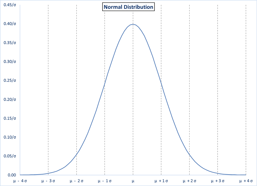
• Here is a typical picture of a normal distribution with known µ and σ. The vertical lines are shown for integer values of z from -4 to 4.

\r\n

The total probability under the curve is 1.00, the total of all possible outcomes. Also, for the normal distribution, the probability of being under any specific part of the curve depends only on z, whatever the values of µ or σ.

Table 4
Normal Distribution Probabilities
z	Pr (X ≤ µ + zσ)
-4	0.000032
-3	0.001350
-2	0.022750
-1	0.158655
0	0.500000
1	0.841345
2	0.977250
3	0.998650
4	0.000068

• The standard normal distribution is the normal distribution with mean = 0 and standard deviation = 1. Any problem involving a normal distribution can be treated as a standard normal problem. The normal random variable, X, can be mapped to a standard normal random value Z, by subtracting µ and dividing the result by σ.

Z = (X- µ)/σ

(7.5.3)

• Any particular value, x, can be similarly mapped in a transformation of formula 7.5.2.

z = (x- µ)/σ

(7.5.4)

Thus,

Pr(X ≤ x) = Pr(Z ≤ z) = NORM.DIST(z,0,1,TRUE)

(7.5.5)

• Excel also has a specific function for the standard normal.

NORM.DIST(z,0,1,TRUE) = NORM.S.DIST(z,TRUE)

(7.5.6)

• In the era before computers, mathematicians would use formula 7.5.4 to map a normal distribution to a standard normal, and then use a printed table of standard normal values, such as all the values from z = -4.99 to 4.99 in increments of 0.01.

7.6. Range and Symmetry

• As essentially already indicated, the range of possible values for the binomial and the hypergeometric is from 0 to some positive integer n. In contrast, the range of possible values for the normal distribution is from -∞ to +∞.
• A normal distribution is always symmetric round the mean. One implication of this is that

NORM.DIST(-z,0,1,TRUE) = 1 – NORM.DIST(z,0,1,TRUE)

(7.6.1)

• The binomial distribution is only symmetric at p = 0.5, and the deviation from symmetry increases as p gets closer to 0 or 1. Similarly, the hypergeometric is only symmetric when M is exactly half of N.

7.7. Normal Approximation to the Binomial

• Mathematicians have proven that if you take random samples of a given size from any population, where the probabilities for each item sampled are identical and independent, the resulting sample averages will be distributed approximately according to the normal distribution. (If you want to know more about this, research the “central limit theorem”.)
• A random sample of size n from a binomially distributed population fits the foregoing criteria. Thus, the binomial probability of x or fewer successes in n trials can is approximated by a normal probability.
• In a binomial with n trials and probability of success for each trial = p, we simply insert the binomial mean and standard deviation for X̄, as provided in Subsection 7.4, into the normal formula as follows

BINOM.DIST(x,n,p,TRUE) ~ NORM.DIST(x/n,p,(p(1-p)/n)0.5,TRUE)

(7.7.1)

Equivalently,

BINOM.DIST(x,n,p,TRUE) ~ NORM.DIST(z,0,1,TRUE)

(7.7.1)

where

z = (x/n – p)/((p(1-p)/n) 0.5)

(7.7.2)

• When using this approximation, one must be aware that the binomial is a discrete distribution while the normal is continuous, as discussed Subsection 7.5 and Footnote 13. The binomial probability of exactly x successes in n trials, is best approximated as the normal probability of being between x – 0.5 and x + 0.5. This is sometimes referred to as a continuity correction.

BINOM.DIST(x,n,p,FALSE) ~ NORM.DIST((x+0.5)/n,p,(p(1-p)/n)0.5,TRUE) – NORM.DIST((x-0.5)/n,p,(p(1-p)/n)0.5,TRUE)

(7.7.4)

• Accordingly, the approximations in Formulas 7.7.1, 7.7.2 and 7.7.3 are more accurately stated as follows

BINOM.DIST(x,n,p,TRUE) ~ NORM.DIST((x+0.5)/n,p,(p(1-p)/n)0.5,TRUE)

(7.7.5)

Equivalently,

BINOM.DIST(x,n,p,TRUE) ~ NORM.DIST(z,0,1,TRUE)

(7.7.6)

where

z = ((x+0.5)/n – p)/((p(1-p)/n) 0.5)

(7.7.7)

7.8. Normal Inverse

• As discussed in Subsection 7.5, the probability that a number drawn from a normal distribution is x or less

Pr(X ≤ x) = NORM.DIST(x,µ,σ,TRUE)

(7.8.1)

• Instead of asking the probability that the number drawn from a normal distribution is x or less, what if we start with a specified probability (prob) and we want to solve for the value of x that results in that probability? Excel offers an inverse that can do this. Solve for x as

x = NORM.INV(prob,µ,σ)

(7.8.2)

• Equivalently, solve for z as

z = NORM.INV(prob,0,1)

(7.8.3)

and then calculate x as

x = z σ + µ

(7.8.4)

• This will be helpful in the next section.

8. Calculating Confidence Levels, Confidence Intervals and Sample Sizes

The most basic approach – the one used that is behind the figures in Tables 1 and 2 in Section 2 – is an approach known as the Wald method. We explain this and then reference some techniques that are generally considered superior.

8.1. Central Region and Tails

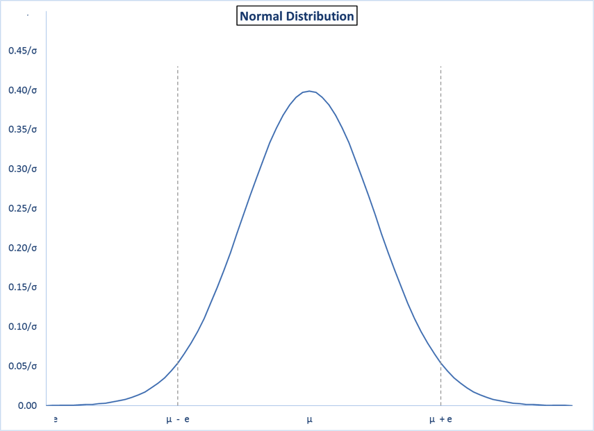
• Assume a normal distribution with known µ and σ. Here is a graph showing a normal distribution with two values, (µ – e) and (µ + e), on either side of µ. This divides the total probability into three areas.

Pr (X ≤ µ-e) = NORM.DIST(µ-e, µ, σ,TRUE)	(8.1.1)
Pr (µ-e ≤ X ≤ µ+e) = NORM.DIST(µ+e, µ, σ,TRUE) – NORM.DIST(µ-e, µ, σ,TRUE)	(8.1.2)
Pr (X ≥ µ + e) = 1 – NORM.DIST(µ+e, µ, σ,TRUE)	(8.1.3)

The total area under the curve represents the total probability of all outcomes. I.e., the total area adds up to 1.00. The middle area – the “central region” – represents the probability of an outcome between (µ – e) and (µ + e). The areas on the left and right are referred to as the “tails”. The size of the left tail represents the probability of an outcome less than (µ – e). The size of the right tail represents the probability of an outcome greater than (µ + e).

• If the distribution is actually binomial with known p and n, and conditions such that Formula 7.7.1 can be used, the three equations can be restated as follows.

Pr (X ≤ p-e) = NORM.DIST(p-e, p, (p(1-p)/n)0.5,TRUE)	(8.1.4)
Pr (p-e ≤ X ≤ p+e) = NORM.DIST(p+e, p, (p(1-p)/n)0.5,TRUE) – NORM.DIST(p-e, p, (p(1-p)/n)0.5,TRUE)	(8.1.5)
Pr (X ≥ p + e) = 1 – NORM.DIST(p+e, p, (p(1-p)/n)0.5,TRUE)	(8.1.6)

8.2. Wald Method

Subsection 8.1 shows that if we know the mean and the standard deviation, we can determine the probability that some observed sample result with be within some interval around the mean. Of course, the problem when sampling is the opposite – we know the observed sample result and we want to quantify the confidence that the actual mean is within some interval around the observed sample result.

We envision two normal curves, one on either side of the observed sample proportion, p̂. p̂ (pronounced “p-hat”) is calculated as p̂= x/n and is an estimate of the actual proportion p.

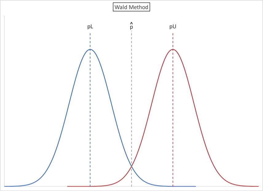
• The mean of the lower curve is pL. This is the lowest value for the mean of a normal distribution that contains p̂ = x/n in its upper tail.

Pr (X ≥ x/n) = (1-CL)/2 = 1 – NORM.DIST(x/n, pL, (pL(1- pL)/n)0.5,TRUE)

(8.2.1)

• The mean of the lower curve is pU. This is the greatest value for the mean of a normal distribution that contains p̂ = x/n in its lower tail.

Pr (X ≤ x/n) = (1-CL)/2 = NORM.DIST(x/n, pU, (pU(1- pU)/n)0.5,TRUE)

(8.2.2)

• The confidence range (confidence interval) is from pL and pU. We know p̂, but we do not know pL and pU. Our goal is to solve for pL and pU.

The Wald Method makes the simplifying assumption that the standard deviation components in Formulas 8.2.1 and 8.2.2 can both be approximated by the known quantity (p̂(1-p̂)/n)^0.5, resulting in the following formulas.

Pr (X ≥ x/n) = (1-CL)/2 = 1 – NORM.DIST(p̂, pL, (p̂, pL, (p̂(1-p̂)/n)0.5,TRUE)

(8.2.3)

Pr (X ≤ x/n) = (1-CL)/2 = NORM.DIST(p̂, pU, (p̂, pU, (p̂(1-p̂)/n)0.5,TRUE)

(8.2.4)

This simplifying assumption also implies that pL and pU are equidistant from p̂ such that

p̂ – pL = pU – p̂

(8.2.5)

• Using the formulas from Subsection 7.5 and Formula 8.2.5, standardize and rearrange Formula 8.2.3 to express pU in terms of n, CL and p̂.

(1-CL)/2 = 1- NORM.DIST(p̂, pL, (p̂(1-p̂)/n)0.5, TRUE)
1 – (1-CL)/2 = NORM.DIST(p̂, pL, (p̂(1-p̂)/n)0.5, TRUE)
1 – (1-CL)/2 = NORM.DIST((p̂ – pL) / (p̂(1-p̂)/n)0.5, 0, 1, TRUE)
1 – (1-CL)/2 = NORM.DIST((pU – p̂) / (p̂(1-p̂)/n)0.5, 0, 1, TRUE)
pU = NORM.INV(1-(1-CL)/2, p̂, (p̂(1-p̂)/n)0.5)	(8.2.6)

• Defining ME = p̂ – pL = U – p̂ as the margin of error, we can further say

pU – p̂ = NORM.INV(1-(1-CL)/2, p̂, (p̂(1-p̂)/n)0.5) – p̂
ME = NORM.INV(1-(1-CL)/2, p̂, (p̂(1-p̂)/n)0.5) – p̂	(8.2.7)

• Similarly, we can express pL in terms of n, CL and p̂.

pL = NORM.INV(1-(1-CL)/2, p̂, (p̂(1-p̂)/n)0.5)	(8.2.8)
ME = p̂ – NORM.INV(1-(1-CL)/2, p̂, (p̂(1-p̂)/n)0.5)	(8.2.9)

• A formula for CL in terms of n, ME and p̂ can also be derived.

CL = NORM.DIST(p̂+ME, p̂, (p̂(1-p̂)/n)0.5, TRUE) – NORM.DIST(p̂-ME, p̂, (p̂(1-p̂)/n)0.5,TRUE)

(8.2.10)

What if we have not yet taken a sample? Instead of using any of formulas 8.2.6 through 8.2.10 as presented above, simply use 0.50 in place of p̂. This will provide conservative results in the sense that ME with be greater, or CL will be lower, than for any other value of p̂. This was the technique used to generate the values in Table 1 in Subsection 2.3. Or, to be less conservative but still conservative, use any value that is closer to 0.50 than the “worst case” anticipated sample proportion.

Finally, when solving for a sample size that will produce a desired CL and ME, one cannot start with a sample average (because that would already depend on having used some sample size.) Thus, solve for n in terms of p, CL and ME and a hypothetical p.

p+ME = NORM.INV(1-(1-CL)/2, p, (p(1-p)/n)0.5)
(p+ME-p)/((p(1-p)/n)0.5)= NORM.INV(1-(1-CL)/2, 0,1)
ME/NORM.INV(1-(1-CL)/2,0,1) = (p(1-p)/n)0.5
(ME/NORM.INV(1-(1-CL)/2,0,1))2 = p(1-p)/n
n= p(1-p)/((ME/NORM.INV(1-(1-CL)/2,0,1))2)	(8.2.11)

Formula 8.2.4 provides the sample size, given a desired CL and ME. The quantity p(1-p) is maximized – and thus the value of n is conservatively maximized – at p = 0.5. By using this maximum sample size, we are sure to meet the desired confidence level and margin of error. This is the basis for Table 2 in Subsection 2.3. If p turns out to be less than 0.5 or more than 0.5, the confidence level will be greater and/or margin of error will be lower.

The Wald method is presented here because it is in common use, but it is generally regarded as inferior to the Wilson and Binomial techniques discussed next. This technique should not be used if n is “too small” or if p is “too close” to either 0 or 1.

We state without proof or mathematical justification that the following constraints should both be satisfied when using the Wald method.

n > 9p/(1-p)	(8.1.12)
n > 9(1-p)/p	(8.2.13)

Thus, if p = 0.10, n should be at least 81. If p = 0.01, n should be at least 891.

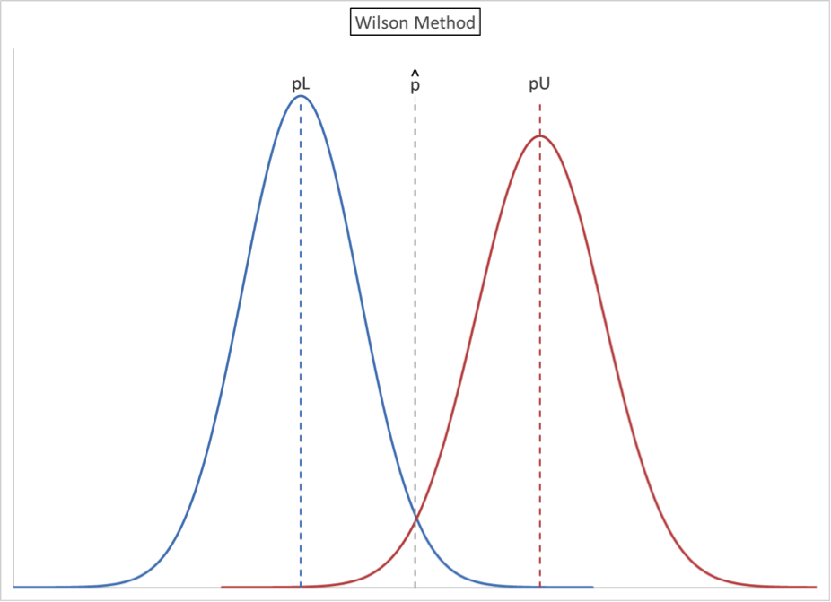
8.3. Wilson Method

In developing a confidence interval using the Wald method, there was a significant simplifying assumption. The assumed standard deviation was based on the observed sample proportion, p̂, and this further implied that pL and pU are equidistant from p̂. The Wilson method again envisions two normal curves, but does not make this simplifying assumption. For this reason, the illustrated curves are different in shape from one another.

In developing a confidence interval using the Wald method, there were two significant simplifying assumptions. The assumed standard deviation was based on the observed sample proportion, p̂ and pL and pU are assumed to be equidistant from p̂. The Wilson method again envisions two normal curves, but does not make these simplifying assumptions. For this reasons, the illustrated are curves are different is shape from one another.

\r\n

• The mean of the lower curve is pL. This is the lowest value for the mean of a normal distribution that contains p̂ = x/n in its upper tail.

Pr (X ≤ x/n) = (1-CL)/2 = 1 – NORM.DIST(x/n, pL, (pL(1- pL)/n)0.5,TRUE)

(8.3.1)

• The mean of the lower curve is pU. This is the greatest value for the mean of a normal distribution that contains p̂ = x/n in its lower tail

Pr (X ≤ x/n) = (1-CL)/2\r\n = NORM.DIST(x/n, pU, (pU (1- pU)/n)0.5,TRUE)

(8.3.1)

• The confidence range (confidence interval) is from pL and pU. We know p̂, but we do not know pL and pU. Our goal is to solve for pL and pU.
• There are formulaic solutions for pL and pU. These involve using the NORM.INV function and then solving a quadratic equation. The solution for pU is as follows, starting with Equation (8.3.2).

(1-CL)/2 = NORM.DIST(x/n, pU, (pU (1- pU)/n)0.5,TRUE)
(x/n) = NORM.INV((1-CL)/2, pU, (pU (1- pU)/n)0.5,TRUE)
(x/n – pU ) = NORM.INV((1-CL)/2), 0, 1) (pU (1- pU)/n)0.5
(x/n – pU )2 = NORM.INV((1-CL)/2), 0, 1)2 (pU (1- pU)/n)
(x/n)2 – 2(x/n) pU + (pU )2 = (NORM.INV((1-CL)/2), 0, 1)2 / n) (pU- pU2)
0 = (pU )2 (1 + NORM.INV((1-CL)/2), 0, 1)2 / n) + pU (-2)((x/n) + NORM.INV((1-CL)/2), 0, 1)2 / n) + (x/n)2	(8.3.3)

Equation (8.3.3) is a quadratic equation in pU, with constants a, b and c.

a = 1 + NORM.INV((1-CL)/2), 0, 1)2 / n	(8.3.4)
b = -2 ((x/n) + NORM.INV((1-CL)/2), 0, 1)2 / n)	(8.3.5)
c = (x/n)2	(8.3.6)

So,

pU = (-b ± (b2 – 4ac)0.5)/(2a)

(8.3.7)

A similar derivation of pL will yield the same result, so pU is the higher root and pL is the lower root.

8.4. Binomial Method

Instead of using two normal curves, as in the Wald and Wilson Method, we can take the same perspective based on two binomial distributions. Instead of calculating a sample proportion, we only need the observed number of “successes”, e.g., x responsive documents in a sample of n documents. The initial equations parallel those of the other methods.

• There is some possible proportion, pL, such that the observed x is the lowest value in the upper tail.

Pr (X ≥ x) = (1-CL)/2 = 1 – BINOM.DIST(x,n,pL,TRUE)

(8.4.1)

• There is some possible proportion, pU, such that the observed x is the highest value in the lower tail.

Pr (X ≤ x) = (1-CL)/2\r\n = BINOM.DIST(x,n,pU,TRUE)

(8.4.2)

• The confidence range (confidence interval) is from pL and pU.
• The goal is to solve for pL and pU. As noted, Excel does not have a binomial inverse function that can be used here.[10. The BINOM.INV function solves for x, not p. The BETA.INV function actually can be used, based on math that relates the binomial function to the beta. Discussion of this theory is beyond the scope of this material, but examples are provided in the accompanying spreadsheet.] Therefore, the typical approach to solving for pL and pU will involve an iterative process. The computer is programmed to “guess” at a value, and based on the results it comes up with it develops another guess. Eventually, the computer gets the value that solves the equation. An example is provided in the accompanying spreadsheet.

The Binomial technique is sometimes referred to as the Clopper-Pearson interval. Because it reflects the actual sampling model and not a normal approximation, it is sometimes also referred to as an “exact” method. One can also apply a Hypergeometric analogue to the Binomial, but this is outside the scope of this material.

8.5. Finite Population Calculations

Subsection 7.4 provides the mean and standard deviation for the average of the binomial distribution. The corresponding values for the average of the hypergeometric distribution, where M is the number of successes and N is the population size, are

Mean: M/N	(8.5.1)
Standard Deviation: ((M/N)(1-(M/N))/n) (N-1/N-n)) 0.5	(8.5.2)

These values can be used in place of the binomial values in the normal approximations in Subsections 8.2 and 8.3 to reflect the finite population impact. Also, HYPGEOM.DIST can be used in place of BINOM.DIST in Subsection 8.4.

8.6. The More Information You Have, the More Precise You Can Be

The most basic approach is to solve for confidence level, margin of error or sample size in term of the other two. When this is done, the math makes the conservative assumptions that (1) the proportion of successes is 0.50, and (2) the underlying population size is infinite.

Greater precision is possible if the actual proportion of successes and/or the size of the finite population are known. The Excel examples help to demonstrate this. The tradeoff is that this requires more intricate math. Over the course of a project, one can start with conservative standard guidelines and evolve toward a more precise picture as more is known.

9. Acceptance Sampling

9.1. Introduction – Zero Defect Testing

Section 3 highlighted an example in which we wanted to establish with 95% confidence that the defect rate in a population of size 2,000 is less than 10%. How big must the sample be such that zero defects in the sample establishes this level of confidence?

Let us first assume the population is infinite or very large, so that the defect rate does not change once a sample is drawn from the population. We define u as the unacceptable defect rate. The probability that any single draw is not a defect is therefore (1-u). The probability of zero defects in two draws is thus

(1-u)*(1-u) = (1-u)2

(9.1.1)

The probability of zero defects in n draws is

(1-u)n

(9.1.2)

The probability of one or more defects in n draws is

1 – (1-u)n

(9.1.3)

If u is 10% in this example, and our approach is to reject the population if there are one or more defects in the samples, we will have 95% confidence of seeing one or more defects if

1 – (1-.10)n ≥ .95

(9.1.4)

Equivalently,

(1-.10)n ≥ (1-.95)

(9.1.5)

With this formulation, we can solve for the lowest necessary n using logarithms.

ln ((1-.10)n) = ln (1-.95)
n ln (1-.10) = ln (1-.95)
n = ln (.05)/ln(.90)
n = -2.99573/(-0.10536) = 28.43316
n = 29	(9.1.6)

In other words, if the defect rate is actually 10%, and we take samples of size 29, we will see at least one defect 95% of the time. If our rule is to accept the lot if we see zero defects, we will incorrectly accept this unacceptable defect rate less than 5% of the time.

We can generalize this problem in two ways. First, instead of specifying a confidence level CL, such as 95%, it is more meaningful to specify (1-CL) as the maximum probability of accepting an unacceptable defect rate, MaxAccUn. Second, recognize that (1-u)ⁿ is the binomial probability of zero observations in a sample of size n if the rate is u. So, Formula 9.1.5 can be stated as

BINOM.DIST(0,n,0.10,TRUE) ≤ 0.05

(9.1.7)

BINOM.DIST(0,n,u,TRUE) ≤ MaxAccUn

(9.1.8)

Because acceptance sampling of this sort will typically involve limited, finite populations, it makes sense to present this relationship using the hypergeometric distributions. Our goal is to find the lowest n such that

HYPGEOM.DIST(0,n,(u*N),N,TRUE) ≤ MaxAccUn

(9.1.9)

Or, specifically in this case, with u = 10%, N = 2000 and MaxAccUn = 5%,

HYPGEOM.DIST(0,n,200,2000,TRUE) ≤ 0.05

(9.1.10)

With the hypergeometric, we cannot use logarithms for a direct solution. The example in the Excel spreadsheet uses a VBA function that searches for n. Table 3 in Section 3 shows some examples.

9.2. Advanced – Limiting the Probability of Incorrect Rejections

The basic problem with the a rule that accepts only on zero defects is that you might find a defect, and thus reject a lot, even though the underlying defect rate is acceptable.

In the example that we have been using, what if the actual defect rate is only 1%, i.e., 20 defects in the population of 2000, and this is an acceptable rate? The probability of one or more defects in a sample of size 29 is

Pr(X ≥ 1) = 1 – Pr(X = 0)	(9.2.1)
Pr(X ≥ 1) = 1 – HYPGEOM.DIST(0,29,20,2000,TRUE)	(9.2.2)
Pr(X ≥ 1) = 1 – 0.7456 = 0.2544	(9.2.3)

In other words, we are happy to have a test that rejects 95% of the time if the defect rate is an unacceptable 10%, but we are not happy that the same test rejects more than 25% of the time even when the defect rate is an acceptable 1%.

This leads to an expansion of the set of definitions.

u = Unacceptable defect rate (as previously defined)

a = Acceptable defect rate

MaxAccUn = Maximum prob of accepting lot with unacceptable defect rate previously defined)

MaxRejAcc = Maximum prob of rejecting lot with acceptable defect rate

x = highest number of defects that will cause us to accept the lot (previously always zero)

n = required sample size (as previously defined)

The task now is to solve for the lowest x, and the associated n, that satisfy both of the following relationships.

• First, as before, the probability of accepting a lot with an unacceptable rate must be at or below the specified maximum.

HYPGEOM.DIST(x,n,(u*N),N,TRUE) ≤ MaxAccUn

(9.2.4)

• Second the probability of rejecting a lot with an acceptable rate must also be at or below the specified maximum.

1 – HYPGEOM.DIST(x,n,(a*N),N,TRUE) ≤ MaxRejAcc	(9.2.5)
HYPGEOM.DIST(x,n,(a*N),N,TRUE) ≥ 1 – MaxRejAcc	(9.2.6)

Now, we are solving for two numbers, x and n, and there is certainly no direct method of calculation. The accompany spreadsheet provides a VBA function that is an array function, meaning that it solves for more than one value. It shows that, in the case where the N = 2000, u =10%, a = 1%, MaxAccUn = 5% and MaxRejAcc = 5%, the testing can be done with a sample size of 61 and a rule that you accept the lot if there up to 2 defects and that you reject the lot if there are more than 2 defects.

10. Examples in the Accompanying Excel Spreadsheet

The accompanying Excel spreadsheet, EDRM Statistics Examples 20150123.xlsm, implements relevant calculations supporting Sections 7, 8 and 9. This spreadsheet was developed using Microsoft Excel 2013.

Notice – This spreadsheet is an .xlsm, meaning that it contains VBA code (macros). You may have to adjust your security settings in order to view and use them.

Caveat– This spreadsheet is intended to assist in learning. EDRM does not warrant the accuracy of this spreadsheet.

• Download EDRM Statistics Examples 20150123.xlsm spreadsheet

There is a Notes page, with same descriptive information that appears here. There are then pages for each of Sections 7, 8 and 9. Basically, these pages provide examples for (most of) the numbered Formulas that appear in those sections.

• Columns with yellow headers are inputs. These can be modified to see results in the other columns.
• Columns with green headers implement the solution using standard Excel formulas and functions. Do not modify these columns unless you specifically intend to modify the logic or implement alternative logic.
• Columns with blue headers implement the solution using Visual Basic for Application (VBA) functions, i.e., “macros”. Do not modify these columns unless you specifically intend to modify the logic or implement alternative logic. Those interested can read the VBA code to see the logic.

Footnotes